Paper Review: Contrastive Sensor Fusion Method and Its Potential Applications to tinyML

This paper talks about understanding remote sensing data through a contrastive sensor fusion method using data from multiple sources.

We will understand why this method is more useful than traditional CNNs and do a deeper dive into their methodology and results. Finally, we will take a look at their biggest takeaways and the potential use cases of this work in the field of tinyML.

Disclaimer: Please note this blog is just covering the paper in a high-level manner. We would encourage you to go into the paper and check out the work from the authors at Descartes Labs.

• Read the paper.
• Download the code.

What is remote sensing data?

This form of data is remote as the word suggests, which means that one does not need to be on site to obtain it. So mostly this data consists of aerial images of several locations around Earth taken from satellites.

So how is remote sensing data different from everyday images collected?

1. They contain a lot of objects or subjects in each image, for example, aerial images can have trees or buildings.
2. Whatever is captured is really small and mutable, which means that images of the same location taken even a few minutes apart can be different.
3. A variety of sensors are combined to get this data and hence images have a variety of resolutions, spectral bands etc.
4. Lastly and what is important in terms of machine learning is that the data is often unlabeled.

But why does unlabelled data pose such a problem in remote sensing?

When we work with any deep learning methods, our models require an abundance of data, especially labelled data for getting good results. With remote sensing images having so many different objects in a single image, labeling is an uphill task.

Previously, researchers have used semi-supervised learning techniques, which first learns on a small amount of labelled data and then expands into unlabeled data.

Semi-supervised learning is particularly successful in remote sensing because it allows you to work with data that are close in time. This theory has a fancy name of “Distributed Hypothesis,” which relies on data being similar in time or space.

However, in this paper, the authors argue that the small changes in data that are assumed by Distributed Hypothesis don’t apply to remote sensing. Most remote sensing images consists of tiny objects like buildings and roads, if we break them into patches, we will find only a few patches that are correlated to each other.

Instead, the authors argue that we need to move towards a representation learning based system, which assumes that similar features on ground should have similar representations regardless of the type of sensors and the combination of sensors involved.

Contrastive methods

Contrastive methods are a widely used form of representation learning. They are used to create representations of  a scene and relate it to another observation in another scene. For example, it is used in Word2Vec where you try to understand words in the same local context or in video processing applications where you can pair frames in the same video.

In the past, contrastive methods were used by taking a small patch from an image and then matching it against another patch in another image.

They were also used to direct the type of sources involved in the training. For example, training images from sensors were used together, making multiple combinations of sensor information.

In this paper, the authors propose a new contrastive method they call CSF, or Contrastive Sensor Fusion, in which you train a single model in an unsupervised fashion, to reproduce the representations of a scene given any sensor and channel combination used during training of that particular scene. The advantage of CSF is that it is not affected by the type or combination of sensors used in the scene. Not just any type of sensors, but combination of sensors or channels as well.

But how is CSF different?

Firstly it doesn’t classify images into patches and match adjacent patches. This would clearly fail in an aerial image, which changes over time. Secondly, since images are captured by multiple sensors that capture different information, the model is forced to look beyond the sensor specific features and instead learn high-level features that are common across all images and sensor combinations.

Apart from this, one of the most interesting parts of CSF is the loss function used: InfoNCE. Unlike autoencoders, which use pixel information like brightness of the image, or filters, we move towards high-level representations. Traditional networks like CNNs examine each pixel and then compare it to the adjacent pixel next to it. Instead, in CSF, we try to create a representation that is the same as a different representation of an image belonging to the same scene but taken from different sensors or combinations of sensors or with channels and pixels dropped out.

CSF and tinyML

Before we dive deeper into the CSF model training methodology and the results from the paper, let us look at how this is applicable to tinyML. One of the primary areas that tinyML targets is the deployment of models to remote areas. We use sensors to capture data and then make a prediction on-device. Since most tinyML devices have a lot of sensors, each with different sensitivities and precision, I believe that the CSF method has the potential to go beyond just remote sensing and aerial images to actual field deployment by combining inputs from multiple sensors to make predictions.

So let us jump into the core of the paper and then look at the possible applications of CSF for tinyML.

How does CSF work?

CSF learns representations. It does this by looking at the high-level information present in the same image from different views.

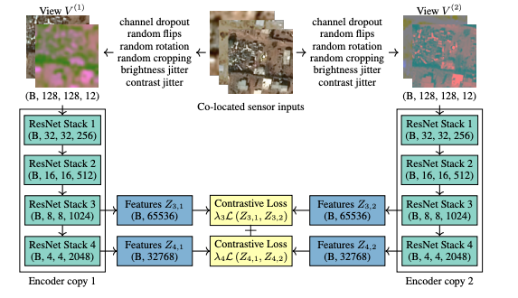
Training is done a little differently, instead of grouping channels separately the network randomly drops out channels, forcing it to learn to encode combinations of channels. Secondly, it allows for weight sharing between encoders and loss at multiple levels of the encoder.

For training the authors created a ResNet 50 encoder and fed it two views. The views are of the same location, but it is different because they have been captured by different sensors or have different brightness, random flips or random channel drops. The two encoders are then trained to create the same output for those different views. In this way the network cannot focus on pixel information but is forced to rely on the information as a whole.

But this begs the question: How does the network discard sensor-based information or is it independent of it?

The training is solely dependent on having multiple views of the data. The authors reinforce the fact that if views differ enough, this forces the encoder to capture high-level information about the scene while foregoing other factors like lightning, resolution and differences between sensors.

While training this network, the authors made sure CSF learns representations of whole images and contrasts representations from distinct scenes rather than patches of a single image.

Takeaways from sensor fusion

In practice, we always know that high-resolution images give better results since they contain more information. We must have encountered that in training our own models, especially in real life settings.

But what exactly happens when you feed the CSF network, low-resolution sensor imagery together with the high-resolution images?

The authors claim that it improves the clustering accuracy, and that multiple low-resolution sensors can outperform a single higher resolution sensor.

The model is trained in an unsupervised fashion, to generate representations. After that they feed in images that are labelled. Using the representations, they train a k-nearest neighbor model.

What do we get from the result?

1. For KNNs of the 10 neighbors, 50.22% is of the same class and the overall accuracy of the entire model is 64.06%.
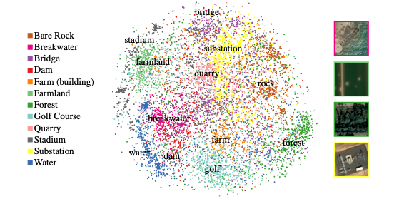
2. They then performed PCA followed by t-SNE and the model has learned representations that have meaning, hence has semantic meaning.
3. Thus showing that it is able to learn these high-level features.

Evaluation of the model

The model is evaluated in the OpenStreetMap object category by how well it are able to cluster scenes. The model’s accuracy is compared to that by ImageNet weights for various sensor/channel combinations

Here, the accuracy is calculated for the representations learned by CSF in comparison to those learnt by ImageNet.

Interesting parts of the result:

1. The CSF encoder is entirely unsupervised whereas the ImageNet encoder requires 14 million labels.
2. When given additional channels, since CSF is an unsupervised model, its accuracy improves.
3. Transfer learning is limited when we fix it at pixel level with low level representations. Since most labelled data is in RGB channels, you cannot take advantage of fusing multiple sensor sources.
4. Images had a fourth channel of infrared, which wasn’t used by ImageNet.
5. Ability to train on multiple low sensor images to achieve greater results than higher resolution images.
6. Order of sensors doesn’t matter, if it is RGB or BGR.
7. The authors argue that as non optical sensors are added, CSF will perform better.

Where will CSF not work?

There are definitely some areas where CSF will be limited.  Areas where semantic classes are complex. Like for example handwriting recognitions, where all the pixels of a particular letter belong to that letter, and hence we need extra transformation to differentiate between classes.

Future work and potential areas of expansion to tinyML

Now that we have understood how CSF works and how it can be useful in multi-sensor applications, let us look into the potential areas of expansion to tinyML.

1. Robustness to lighting conditions: Most tinyML systems are deployed to places where conditions are different from what the model was trained with. One major factor that can affect accuracy is the lighting throughout the day. CSF can be used to train on some of the labelled data of such lightning conditions and it could still have the capability to make predictions in low lighting conditions.
2. Pixel damages on camera: Imagine you are deploying your edge computing systems in a rough environment. Cameras are prone to dust or dirt particles. Since the network is based on representations and not pixels, the accuracy should not be affected.
3. Predictive maintenance: Combine data from accelerometer, gas sensor, microphone, camera, pressure sensor etc to train a model which is completely unsupervised, and deploy it anywhere with any combination of sensors and it will still work. The system will still work if some sensors get damaged.
4. Graceful degradation: Since CSF can work with any combination of sensors, we can build a system that degrades gracefully when it is running low on battery by shutting down sensors that consume more power, while still maintaining good accuracy.