
FOMO™ is a deep learning architecture for running object detection on constrained devices, developed by Edge Impulse.
It combines an image feature extractor ( by default, a truncated section of MobileNet-V2) with a fully convolutional classifier to frame object detection as object classification over a grid, run in parallel.
Read more about FOMO in the Edge Impulse documentation: https://docs.edgeimpulse.com/docs/edge-impulse-studio/learning-blocks/object-detection/fomo-object-detection-for-constrained-devices
Localized object detection
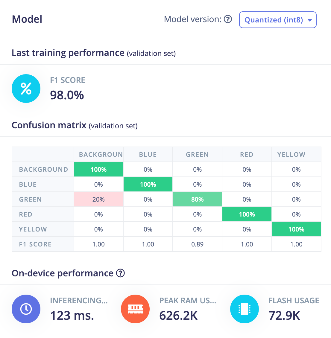
Consider an example of detecting different colored cubes on a conveyor belt: https://studio.edgeimpulse.com/public/230968/latest
FOMO does very well at this class of problem; it’s a perfect fit where object detection can be framed as object classification in a grid since all that is required for each classification is localized to that section of the input.
Fun fact: This is the project FOMO was originally developed on!
Spatial aware object detection
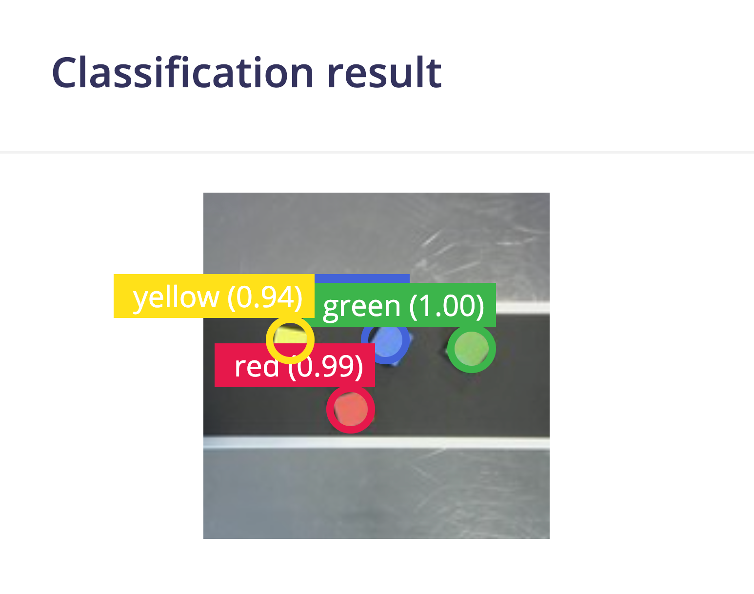
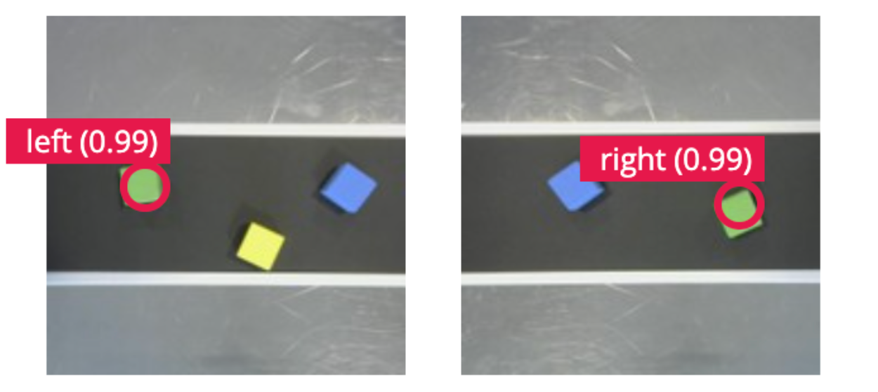
Now consider the same set of input images, but we instead focus on just the green cube and try to predict, not based on color, but based on whether the cube is to the left of other cubes, or to the right.
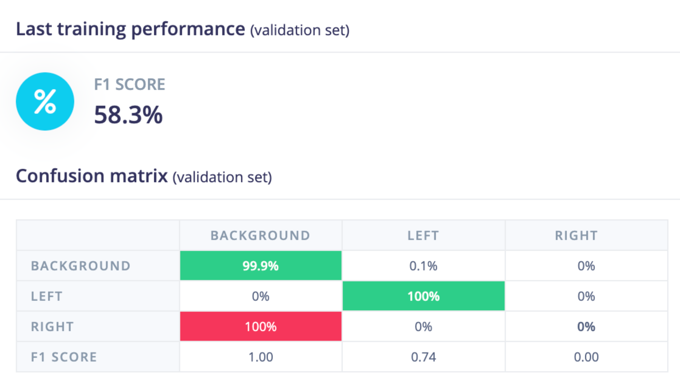
This is not something FOMO can do well. While it is able to identify background vs the green cube in general, it doesn’t know whether the cube is the left or right of others so instead just makes a decision to label them all as left.
To make this work we need to add some spatial understanding to FOMO, but before we do let’s review how FOMO is structured.
Architecture review
By default, the FOMO architecture consists of two fundamental pieces
- a MobileNet-based feature extractor, though any feature extractor can be used, and,
- a fully convolutional classifier.
For the sake of a concrete example let’s consider a specific configuration of
- an image input of size (160, 160, 3)
- a MobileNet-V2 (truncated) backbone with alpha=0.35
- the default configuration for the FOMO fully convolutional classifier ( i.e. a dense connection with 32 units )
- and a binary classifier output
In this scenario, we have the following intermediate shapes and learnable parameters.
 layer                     tensor shape         #parameters  comment
 input                     (None, 160, 160, 3)  0            input
 MobileNet-V2 backbone     (None, 20, 20, 96)   15,840       image feature extractor
 dense (Conv2D)            (None, 20, 20, 32)   3,104        fully convolutional classifier
logits (Conv2D) (None, 20, 20, 2) 66 fully convolutional classifier 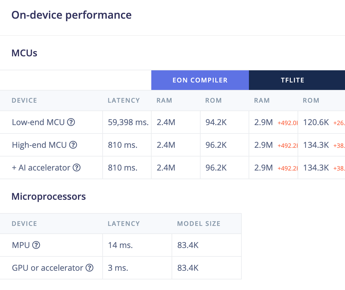
Integrating spatial information with a micro transformer
One effect of acting fully convolutionally on the extracted feature map is that there is no integration of information over the entire input; a detection in an area on "one side" of the input is no different from one from the "other side".
For many problems this is the desired behavior, hence was a core FOMO design decision, but as we’ve just seen in the previous example it isn’t always. Sometimes we need to include some signal that incorporates where in the image the detection is occurring in relation to other objects.
One approach to incorporate this spatial information is to include a minimal transformer block between the feature extractor and the classifier. To support this we’ve added some custom layers to our libs available in Expert Mode WithSpatialPositionalEncodings and PatchAttention
WithSpatialPositionalEncodings takes a feature map (batch, height, width, channels)and adds a spatial form of positional encodings, as additional channels, across the entire feature map. These positional encodings are a 2D form of the normal linear sin/cosine encodings so that the model can use them to incorporate spatial information. Adding this kind of positional encoding is standard before self-attention since self-attention would be otherwise permutation invariant.
PatchAttention converts the 3D spatial array of (height, width, channels) into a 2d array of just (height*width, channels) and then applies MultiHeadAttention.
These two layers can be incorporated in a number of ways but the most straightforward is to add them to FOMO as a branch. We do this as a branch since it allows the main flow to continue to be from the feature extractor to the classifier but allows the optimization to mix in extra spatial information as it requires it from this attention block. Note: we include an aggressive dropout at the start of this branch since self-attention can overfit.
# Cut MobileNet where it hits 1/8th input resolution; i.e. (HW/8, HW/8, C)
    cut_point = mobile_net_v2.get_layer(’block_6_expand_relu’)
    model = cut_point.output
# Now attach a small additional head on the MobileNet
model = Conv2D(filters=32, kernel_size=1, strides=1,
               activation=’relu’, name=’head’)(model)

# Branch, attend (with positional encodings),
# and recombine as residual connection
from ei_tensorflow.self_attention import WithSpatialPositionalEncodings
from ei_tensorflow.self_attention import PatchAttention
from tensorflow.keras.layers import Dropout, Add
branch = Dropout(rate=0.5)(model)
branch = WithSpatialPositionalEncodings()(branch)
branch = PatchAttention(key_dim=8)(branch)
model = Add()([model, branch])

# And finally a classifier layer
logits = Conv2D(filters=num_classes, kernel_size=1, strides=1,
                activation=None, name=’logits’)(model)
return Model(inputs=mobile_net_v2.input, outputs=logits)</code></pre><p>This results in a model with the following intermediate shapes and learnable parameters.</p><pre><code class="language-plaintext"> layer                               tensor shape         #parameters  comment
This gets a bump in performance now getting 4 of 5 "left" instances and 1 of 2 "right" instances in validation data.
A public version of this project is available here: https://studio.edgeimpulse.com/public/230985/latest
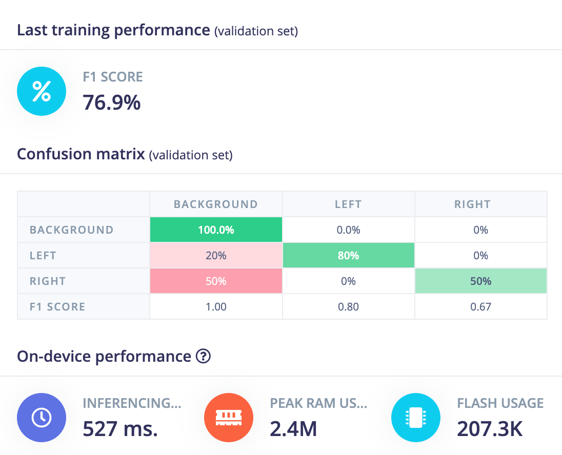
It also now correctly identifies two examples in held-out test data.
The performance comes with a cost, though, primarily around the extra allocation required for the positional encodings.
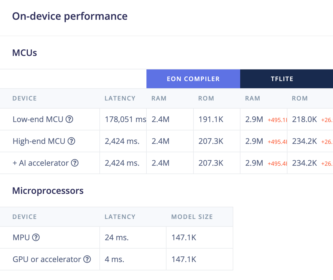
If we wanted to tune further one key option is to control the amount of information being passed to the self-attention block with a projection. For example, projecting down to a lower dimensionality at the start of the branch, then back to the original dimensionality at the end, results in an overall reduction in parameters, even though it introduces two extra layers for the projections. In some cases forcing the self-attention to work with a lower dimension representation works as a better regulariser than a dropout.
# Branch, attend (with positional encodings),
# and recombine as residual connection
from ei_tensorflow.self_attention import WithSpatialPositionalEncodings, PatchAttention
from tensorflow.keras.layers import Add
def projection(dim):
  return Conv2D(filters=dim, kernel_size=1, strides=1,
                kernel_initializer='orthogonal',
                use_bias=False)
branch = projection(dim=4)(model)
branch = WithSpatialPositionalEncodings()(branch)
branch = PatchAttention(key_dim=16)(branch)
branch = projection(dim=32)(branch)
model = Add()([model, branch])
layer tensor shape #parameters comment
input (None, 160, 160, 3) 0 input
MobileNet-V2 backbone (None, 20, 20, 96) 15,840 image feature extractor
dense (Conv2D) (None, 20, 20, 32) 3,104
dense (Conv2D) (None, 20, 20, 4) 128 down projection
with_spatial_positional_encodings (None, 20, 20, 4) 0 self attention branch
patch_attention (None, 20, 20, 4) 316 self attention branch
dense (Conv2D) (None, 20, 20, 32) 128 self attention branch
logits (Conv2D) (None, 20, 20, 3) 99 fully convolutional classifierIn this case, the two projections add 256 learnable parameters, but the attention parameter count drops from 1,144 to 316 so it’s a net saving.
Getting started
The easiest way to get started with this idea is to visit this public project and use the expert mode code as an example to start from. Let us know if there are cases where you see an interesting result!