
Introduction
Production lines are fast-paced environments. The ability to detect manufacturing or packaging defects before shipping is critical to improving delivery and customer satisfaction. However, automated inspection equipment needs to process and make decisions without slowing the production line. This is where equipment such as the Kria K26 System on Module (SoM) from Xilinx can help.
The Kria K26 SoM (Figure 1) allows developers to leverage the parallel nature of programmable logic combined with high-performance Arm processor cores. What is exciting about the Kria SoM is that for the first time, Xilinx provides the heterogeneous SoC and the necessary supporting infrastructure for the SoC (XCK26), such as 4GB DDR4 Memory, 16GB eMMC, 512Mb QSPI, TPM Security module, and the necessary power infrastructure.

To make it easy to interface with your application, dual 240-pin connectors are provided that break out 245 IO.
Xilinx also offers the Kria KV260 Vision AI Starter Kit to enable developers to get started and hit the ground running. The kit provides developers with a carrier card for the SoM, which offers the following interfaces:
- 3 MIPI interfaces
- USB
- HDMI
- Display port
- 1 GB Ethernet
- Pmod
This starter kit also comes with a range of applications that show how easy it is to get started developing vision-based artificial intelligence applications. This makes the Kria Vision AI Starter Kit perfect for the applications where fast image processing is required, such as detecting whether or not a label has been correctly applied to a shipping box on the production line.
Manufacturing application use case
Let’s look deeper at how the Kria KV260 Vision Starter Kit can be used for a manufacturing application. Creating a manufacturing application is not necessarily going to require any programmable logic design. However, it will require software development and the ability to train and compile a new machine-learning model using Vitis AI from Xilinx. The first step is installing and configuring Vitis AI for use.
Bill of materials
- Kria KV260 Vision AI Starter Kit
Creating a virtual machine
Running Vitis AI requires either a Native Linux machine or a Linux Virtual Machine running one of the supported Linux Distributions.
Creating a Virtual machine that can run Vitis AI is simple. First, download the Oracle Virtual Box.
Once the virtual box is installed, download the Ubuntu Linux disk image that can be used to install Linux on the virtual machine. The version of Ubuntu used for this project is Ubuntu-18.04.4 Desktop-amd64.iso available here.
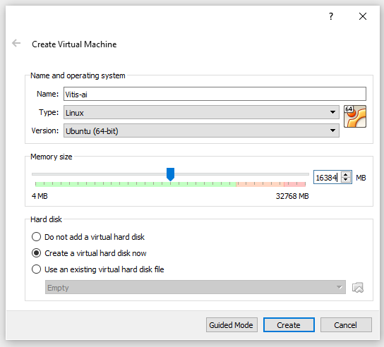
We are now able to build the virtual machine. The first step is in the virtual box manager to click on New.
This will present a dialog that enables the creation of the new VM (Figure 2). Enter a name for the VM and select the type as Linux and version as 64-bit Linux. We can also decide how much system memory is needed to share with the virtual machine (Figure 3).
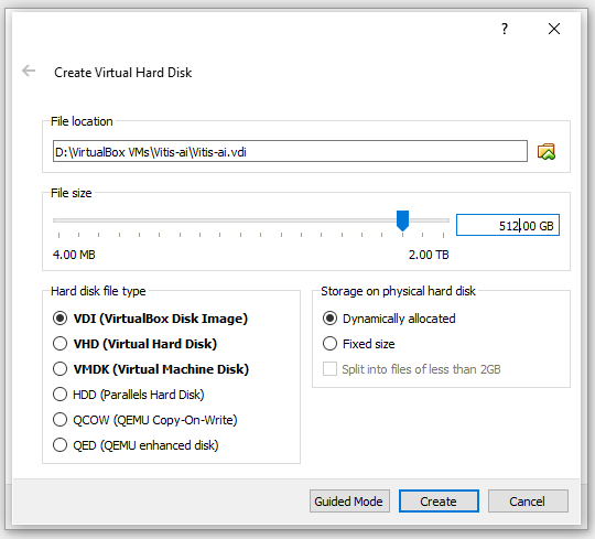
Click on the create button, and the settings for the virtual hard disk will be presented. Select 512GB, which allows the physical storage to be dynamically allocated. The Virtual Hard Disk size will expand to 512GB as disk usage increases. This project was developed using an external solid-state USB C drive to store the Virtual Hard Disk to ensure the space available.
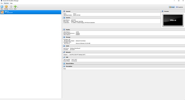
With the VM configured, the next step is to install the operating system. With the newly created VM selected, click on the start button to fire up the VM 9 (Figure 4).
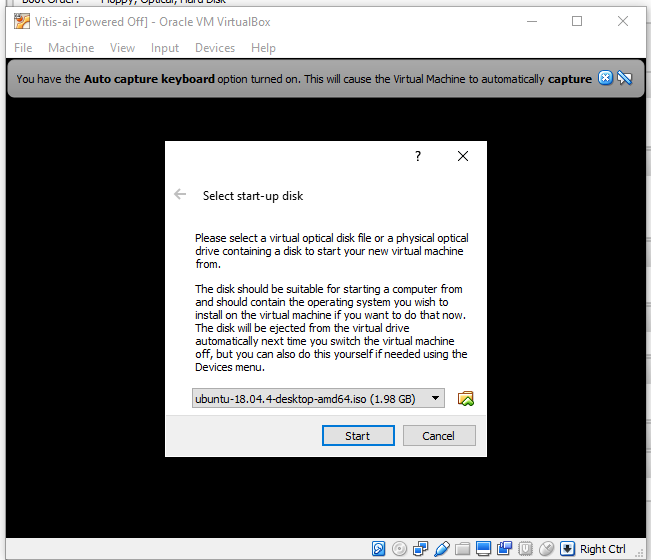
As the VM starts, it will ask for the Ubuntu ISO downloaded previously (Figure 5).
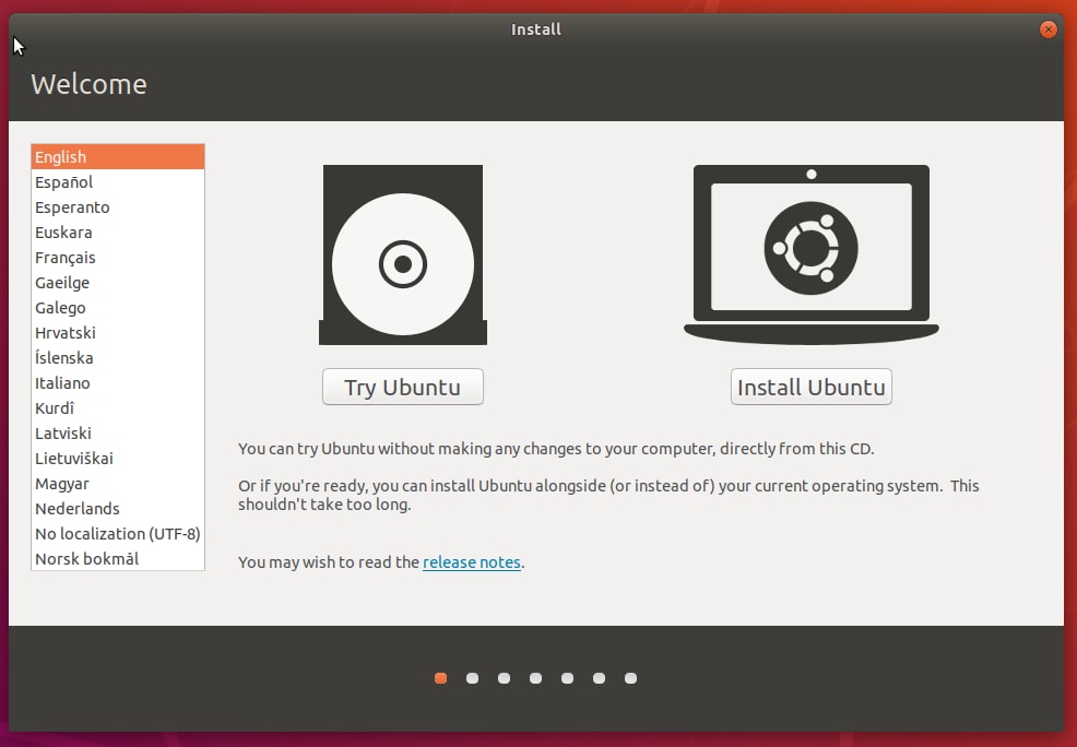
The next steps are to install the Ubuntu operating system on the virtual hard disk. Select install Ubuntu (Figure 6).
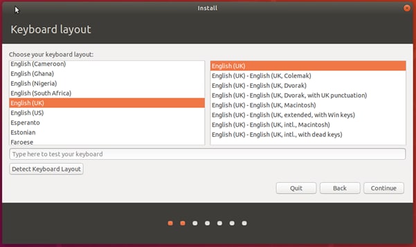
Select the options as to location and configuration of Ubuntu. Select the keyboard configuration (Figure 7).
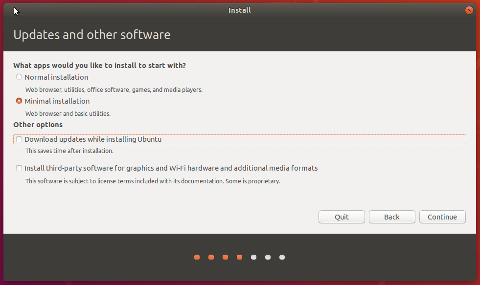
Select minimal installation (Figure 8) as we will not use office software, media players, or games.
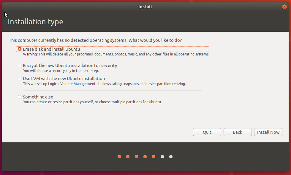
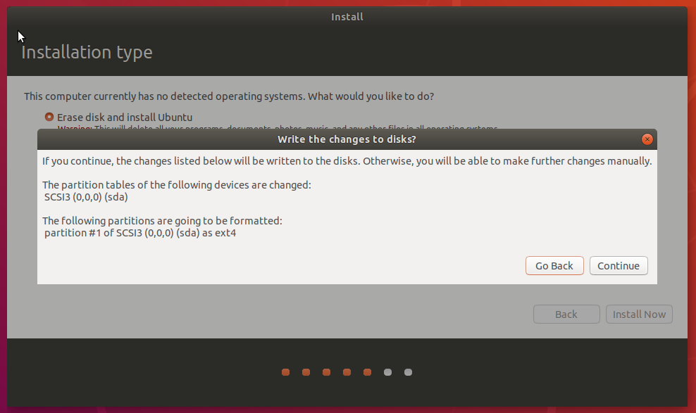
Allow the installation process to erase the disk and install Ubuntu (Figure 9).
Click continue to proceed with the changes (Figure 10).
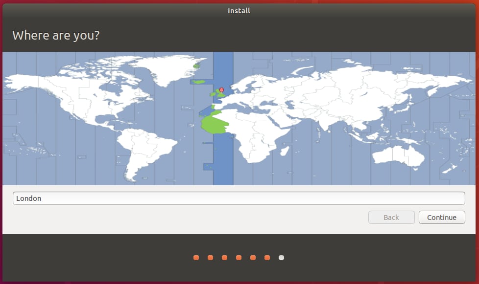
Select your location and time zone (Figure 11).
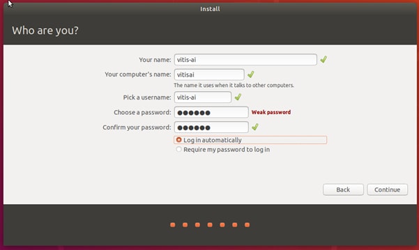
Finally, enter the Ubuntu computer name, username, and password (Figure 12).
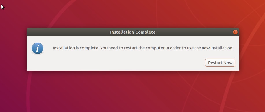
Finally, once the installation is completed, restart the virtual machine (Figure 13).
Once the VM restarts, log in and start installing Vitis AI (Figure 14).

Installing Vitis and Vitis AI
With the Virtual Machine running Linux, our next step is to install both Vitis and Vitis AI. You will need a Xilinx user account to install Vitis, which can be created as part of the download process. As Vitis is the longer of the two installs, we will start with that first.
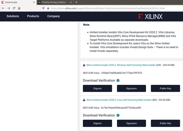
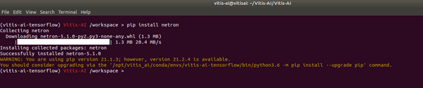
Go to the Xilinx downloads page and select the Linux Self Extracting Web Installer (Figure 15).
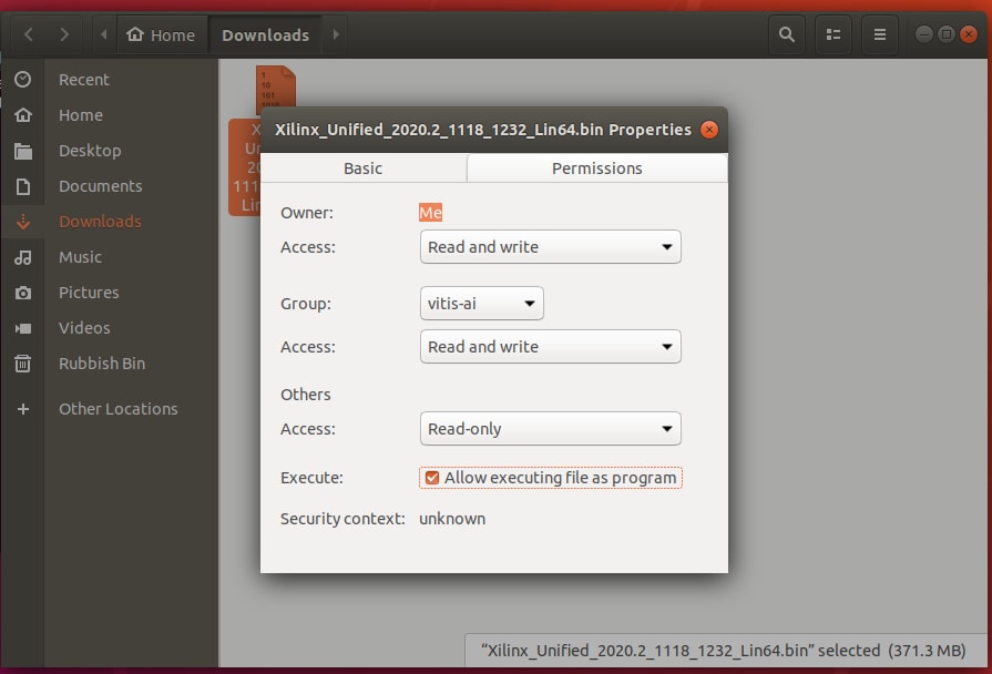
With the web installer downloaded, navigate to the download location, select the application, and right-click it to change its permissions to enable it to be executed as an application (Figure 16).
We can now use a terminal window to install Vitis. This might take time depending upon the capabilities of your VM and internet connection.
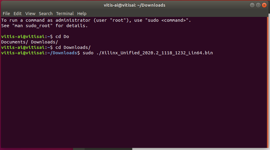
Use sudo to install the tool with the command (Figure 17).
sudo ./Xilinx_Unified_2020.2_1118_1232_Lin64.bin
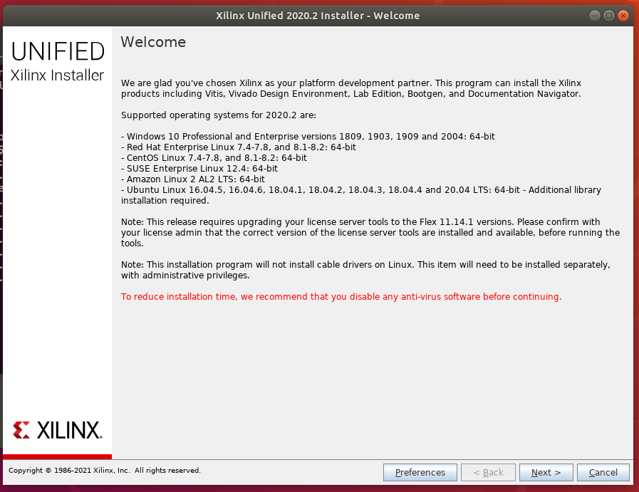
This will start the Vitis Installer (Figure 18).
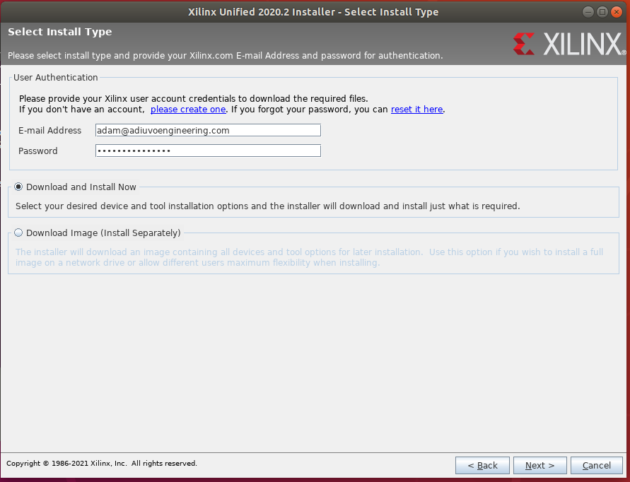
Sign in to your account (Figure 19).
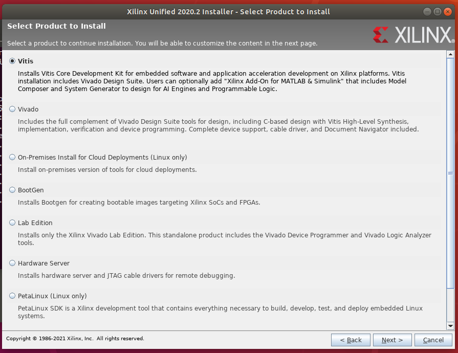
Select Vitis as the target application. This includes Vivado (Figure 20).
To reduce the installation size, uncheck all devices but the SoCs (Figure 21).

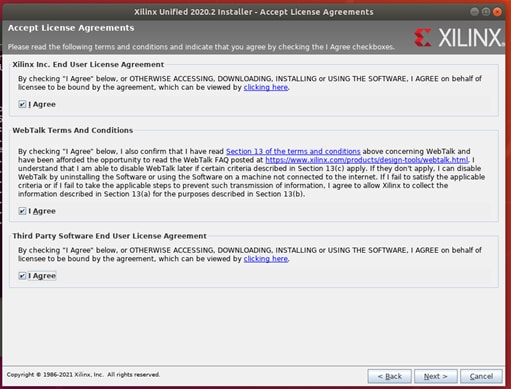
Agree to the terms and conditions (Figure 22).
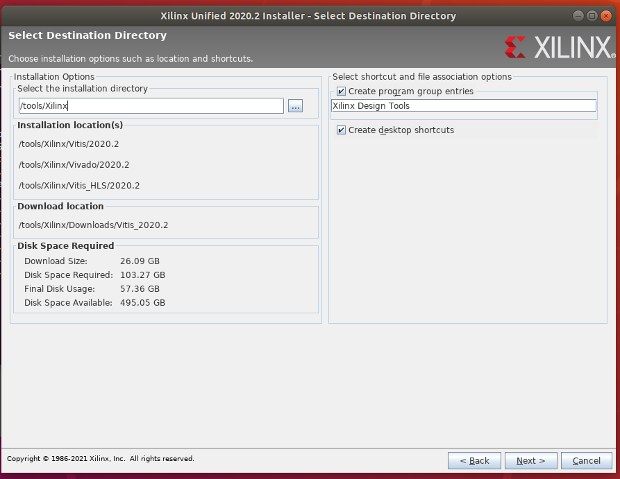
Select the installation directory. I suggest leaving it as default (Figure 23).
On the installation summary, select install and wait (Figure 24).

Once the installation is complete, we need to run the script below to install all the dependencies:
sudo <install_dir>/Vitis/<release>/scripts/installLibs.sh
The next step is to install Vitis AI. In this instance, we will install Vitis AI to run from the CPU and not the GPU, which will mean slower training performance.
The first step is to install docker. This can be achieved following the instructions here. Note, it might be necessary to restart the Virtual Machine once this has been completed.
The following steps are to install Git using the commands:
sudo apt update
sudo apt install git
Select/create a directory to install Vitis-AI clone the Vitis-AI using the command:
git clone
https://github.com/Xilinx/Vitis-AI.git
Once the Vitis-AI repository has been cloned, the next step is to change the directory into it and pull the docker image.
cd Vitis-AI
docker pull xilinx/vitis-ai:latest
This will take several minutes to download the latest Vitis-AI image from docker.
After the docker image has been pulled, we need to build the cross-compilation system. We can do this by running the script located under Vitis-AI/setup/mpsoc/VART (Figure 25).
cd Vitis-AI/setup/mpsoc/VART
./host_cross_compiler_setup_2020.2.sh
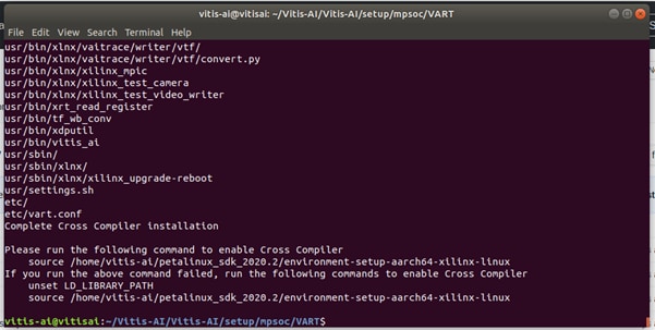
Once the script has run, be sure to run the indicated command to enable the cross-compilation environment.
We can test if we have installed Vitis AI correctly by compiling one of the demonstration programs. In this case, the resnet50 application provided under the demo/VART/Resnet50 directory. To build the application, use the command:
Bash -x build.sh
Provided you see no errors reported in the terminal window and the executable appears in the directory, the Vitis AI installation is working (Figure 26):

Now we need to start developing the dataset that shows the labels correctly and incorrectly applied.
Creating the dataset
To train a neural network, we first need a dataset of correct and incorrect images. To do this, several boxes were applied with the Mouser labels both correctly and incorrectly. To have a diversity of images, both the correct and incorrect boxes were photographed from several angles (Figures 27 and 28).
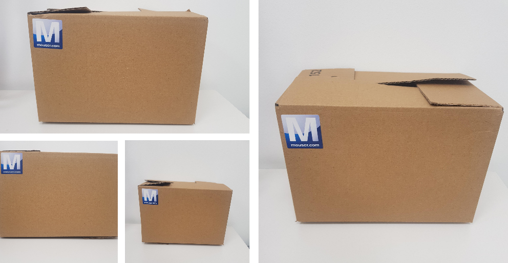
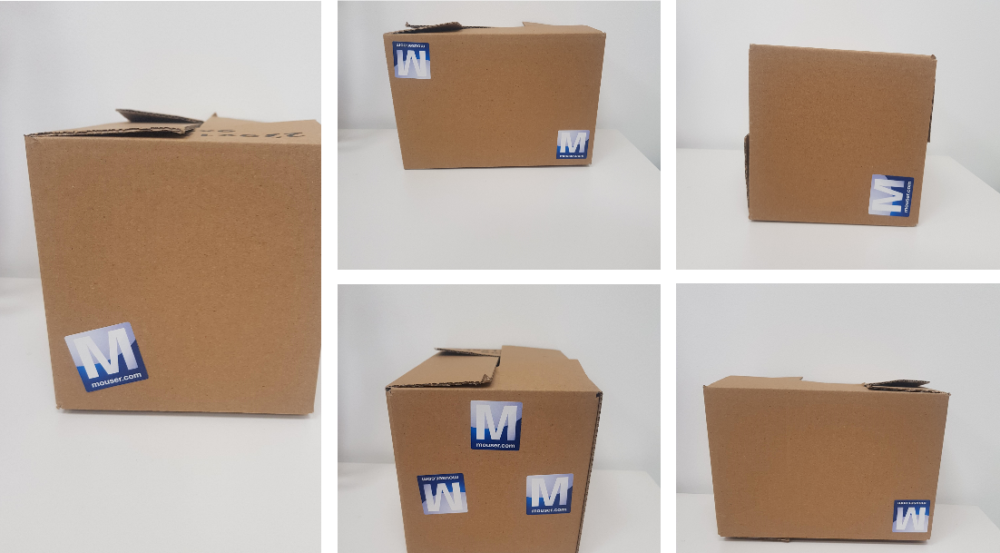
The images were collated into two directories - one for the correct label and another for the incorrect label.
With the images captured, we need to train a neural network. To do this, I will use Edge Impulse to train the neural network as it makes the training easy. Note that you will need to create an account for Edge Impulse, but it is free.
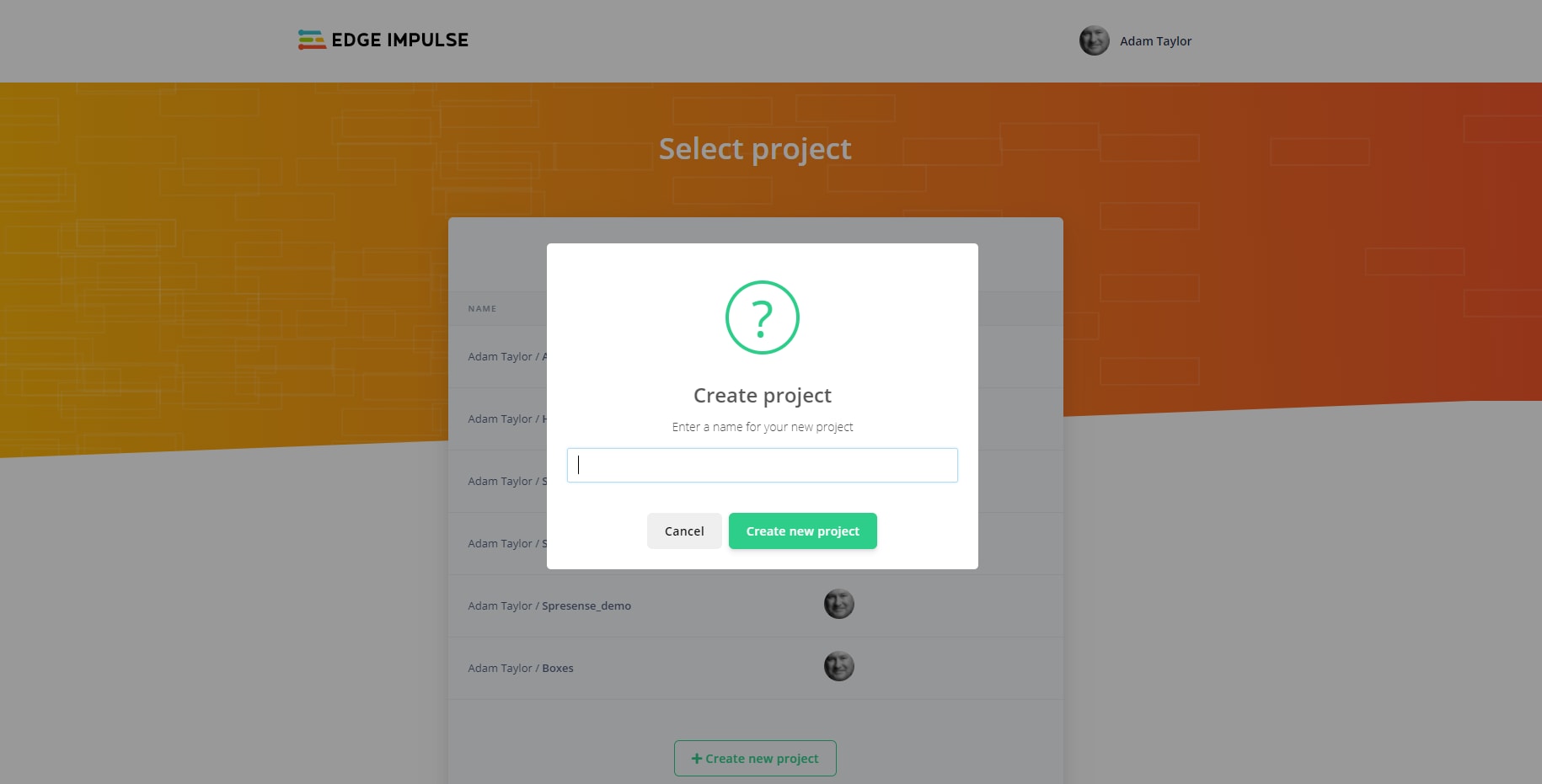
In Edge Impulse, the first thing to do is create a new project (Figure 29).
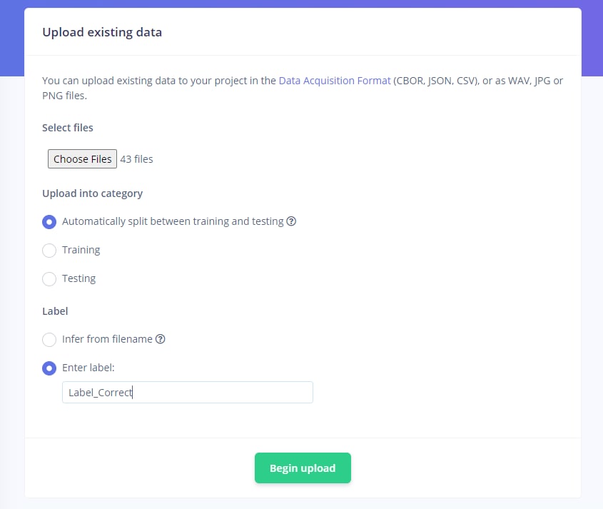
Once the new project has been created, we can upload the images folders, labeled as correct and incorrect. Select all of the files first in the correct directory and upload with the label Label_Correct. After upload of the correct images, upload the incorrect images and label them Label_Incorrect (Figure 30).
With the images all uploaded, the next step is to define the impulse. Select an input image width and height of 224px in each direction. Select an image input and then the Transfer Learning. Save the impulse (Figure 31).

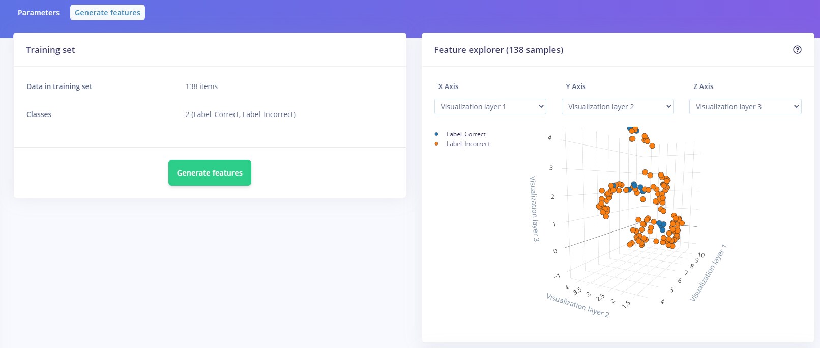
We can then train the model, by generating the features and training the impulse (Figure 32).
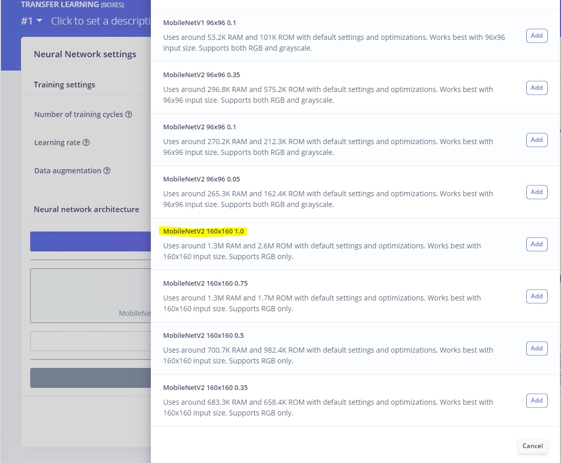
Select the model MobileNetV2 160x160 1.0. An equivalent model is in the Xilinx Model Zoo (Figure 33).
Train the model. This might take a few minutes. Once the model has been trained, go back to the overview page and select the download transfer learning model (Figure 34).
This will include the saved model and the variables (checkpoint) in a .zip file.
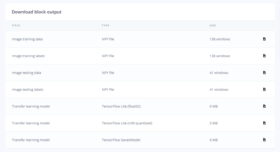
Figure 34: Downloading the saved model
Quantizing and compiling the model
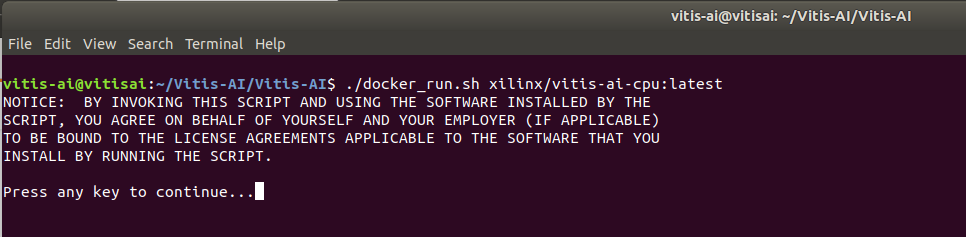
The next step is to quantize and compile the model using Vitis AI. In the virtual machine, we can run Vitis AI by issuing the following command (Figure 35).
./docker_runs.sh Xilinx/vitis-ai-cpu:latest
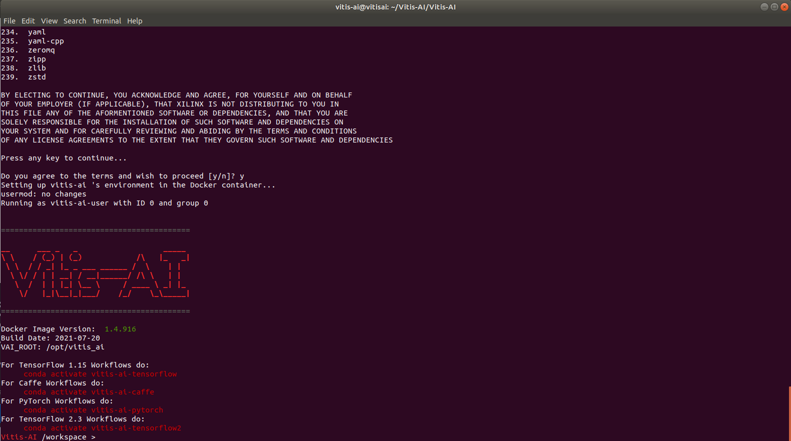
With Vitis AI loaded, activate TensorFlow with the command (Figure 36).
conda activate vitis-ai-tensorflow
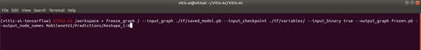
The next step is to freeze the model that merges all the information from the checkpoint into the frozen model file (Figure 37).
Once the model has been output as a frozen model, we can use the compiler to compile the output model so that we can deploy it on the system.
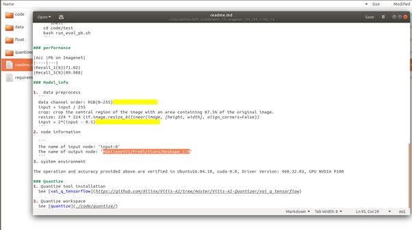
We can learn the information of the output nodes from the YAML file contained within the Xilinx Model Zoo (Figure 38).
To inspect the frozen netlist, we can install Netron. It is important to understand the input and output nodes names for the quantization process (Figure 39).
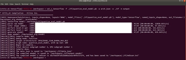
With a quantized netlist available, we can compile the quantized netlist to a model deployed on the Kria SoM (Figure 40).
vai_c_tensorflow -f /quantized_model.pb -a arch.json -o ./tf -n Output
Using SCP/FTP, we can upload the compiled model to the Kria file system under:
/usr/share/vitis_ai_library/models/
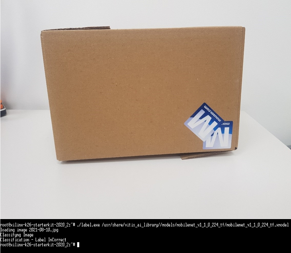
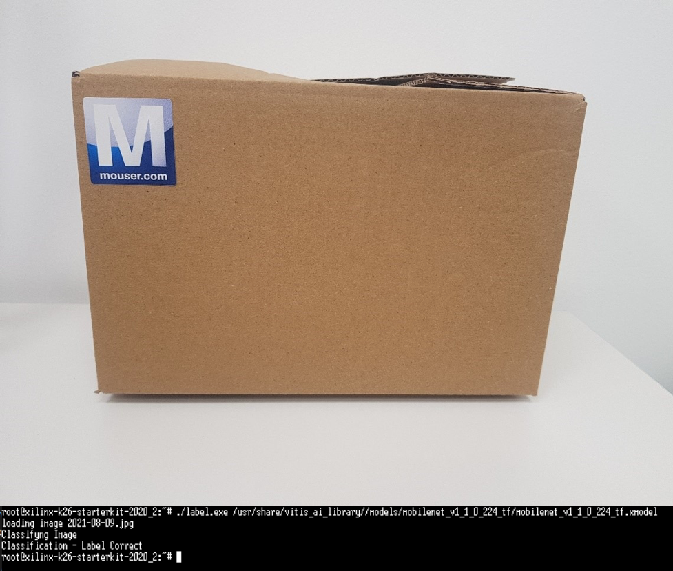
With the model uploaded, we can generate a software application that can be used to test the neural network. To do this, several correct and incorrect images are uploaded to the Kria SoM and used to test the application (Figure 41 and 42).
Wrap up
This project has shown how easily a neural network can be trained and deployed in the Kria SoM for industrial AI / ML applications. The potential is limitless. Future adaptations could be to update the software to utilize the gstreamer framework and classify images live as they would be on the production line.
This article was first published on the Mouser blog.