
As a general philosophy, the Edge Impulse platform aims to provide a developer the functionality they need, with sensible defaults, for common edge AI tasks and focuses on extensibility to handle the rest. One such example of this is with anomaly detection.
Built into the Edge Impulse platform, there are two approaches to non-visual anomaly detection: k-means and Gaussian Mixture Models (GMM). The challenge is that neither one of these methods works well on unprocessed time-series data; they require extracted features or tabular data to be effective. The solution? A custom anomaly detection learning block using an alternative approach.
In this post, we’ll walk through why the k-means and GMM algorithms fail on unprocessed time-series data, how you can create your own custom anomaly detection learning block, and discuss the benefits of a convolutional autoencoder architecture for time-series data anomaly detection.
Benefits of k-means and GMM
The two anomaly detection methods currently available in the Edge Impulse platform, k-means and GMM, remain the default approaches for good reason. When applied to well-structured feature representations, such as FFTs or statistical summaries, they are simple, fast, and highly effective.
They require only minimal non-anomalous training data, have low computational overhead, and map cleanly to resource-constrained edge deployments. For many common anomaly detection tasks, especially where meaningful features can be extracted, these methods provide a strong baseline with predictable behavior. The challenge isn’t that these algorithms are fundamentally flawed, but that unprocessed time-series data does not naturally fit the assumptions they rely on, which becomes particularly apparent when applying them directly to raw sensor data.
Challenges with k-means and GMM
k-means and GMM are both clustering-based approaches that assume your data can be grouped into regions of similarity based on distance. In k-means, this involves assigning samples to the nearest centroid; in GMM, it involves estimating the probability that a sample was generated from a particular Gaussian distribution. In both cases, the underlying assumption is the same, similar data points are close together in feature space, and distance is a meaningful proxy for similarity.
This assumption starts to break down when you apply these methods directly to unprocessed time-series data. A single window of time-series data, say a short segment of sensor readings, becomes a high-dimensional vector where each reading is treated as an independent feature. In high-dimensional spaces, distance metrics become less informative as many points begin to look equally far apart, making it difficult for clustering algorithms to form stable, meaningful groupings. This is a classic manifestation of the “curse of dimensionality,” and it directly impacts how well k-means and GMM can separate normal from anomalous behavior, often producing clusters that are either too broad or overly sensitive to small, irrelevant differences.
Beyond dimensionality, these methods also struggle because they treat time-series data as flat vectors, relying on element-wise comparisons where each data window must align exactly. In practice, signals often contain patterns that can shift slightly in time, such as a spike or waveform occurring a few samples earlier or later, without changing the underlying behavior. Distance-based methods like k-means and GMM have no notion of this and will treat these shifts as meaningful differences, even when they are not. This makes them highly sensitive to minor variations in temporal alignment and limits their ability to group together signals that are structurally similar but not perfectly synchronized.
Raw signals also tend to be noisy, exhibit drift, or vary in amplitude over time. These effects can further complicate distance-based approaches, especially when working in a feature space where small variations may be overemphasized. Without careful normalization or preprocessing, this can lead to unstable clusters or overly broad distributions that blur the boundary between normal and anomalous data.
Because of these limitations, k-means and GMM typically rely on feature engineering to be effective for time-series tasks. Transformations such as FFTs, statistical summaries, or domain-specific features convert raw signals into a more compact and structured representation where similarity is more meaningful. While effective, this adds an extra layer of complexity and reduces flexibility when working across different signals or domains.
Custom anomaly detection learning blocks
While k-means and GMM are the default anomaly detection methods in Edge Impulse for non-visual tasks, they are fortunately not the only option. The platform is designed to be extensible, allowing you to bring your own approaches into Studio through custom learning blocks. This capability is available to both enterprise users and those on the free developer tier, so you’re not limited to pre-defined algorithms when your use case requires something different.
Custom learning blocks let you define your own model architecture and training pipeline, and integrate it directly into the standard Edge Impulse workflow alongside built-in options. This extensibility also applies to anomaly detection, enabling you to plug in alternative models or methods that better fit your data rather than relying on a fixed algorithm.
If you’re interested in building your own, the custom learning blocks documentation covers the structure and interface in more detail.
And that’s exactly what we did here. Alex Elium, an engineer on our Applied Research team, created a custom anomaly detection learning block using a 1D convolutional autoencoder architecture, an approach that operates directly on unprocessed time-series data and avoids many of the limitations we just discussed.
A convolutional autoencoder approach
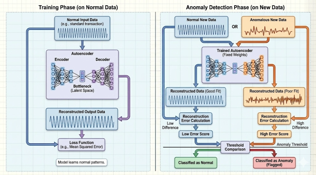
Rather than clustering points in feature space, a convolutional autoencoder takes a fundamentally different approach; it learns a model of normal behavior directly from the data itself.
At a high level, an autoencoder is trained to reconstruct its input. It consists of two parts: an encoder that compresses the input into a lower-dimensional representation, and a decoder that reconstructs the original signal from that compressed form. During training, the model only sees normal data and learns an efficient representation of those patterns. When it encounters new data, it attempts to reconstruct it in the same way. If the input is similar to what it has seen before, reconstruction is accurate. If not, the reconstruction error increases. This error becomes the signal used for anomaly detection.
This approach offers several key advantages over clustering-based methods like k-means and GMM.
First, it avoids the limitations of distance-based methods in high-dimensional spaces. Instead of relying on distances between vectors, the autoencoder learns a compressed representation that captures the most important structure in the data. By forcing the model through a bottleneck, it effectively performs its own feature learning, extracting only the patterns necessary to reconstruct normal behavior. This allows it to operate directly on unprocessed time-series data without requiring hand-engineered features.
Second, the model is able to learn and represent complex, non-linear patterns. Real-world signals often contain combinations of trends, periodicities, and subtle variations that are difficult to capture with simpler approaches like k-means and GMM, which rely on distance and distributional assumptions. Deep learning-based approaches, including autoencoders, are well-suited for modeling these kinds of structures and can better handle the non-linear and noisy nature of real time-series data.
Third, anomaly detection becomes a byproduct of reconstruction rather than clustering. Instead of asking “which cluster does this belong to?”, the model asks “how well can I explain this signal?” This shift reframes the problem from partitioning space to modeling behavior. As a result, the model can detect anomalies that don’t simply fall far from a centroid, but instead violate learned patterns in more subtle ways.
The use of 1D convolutional layers further strengthens this approach for time-series data. Convolutions apply small filters that slide over the signal, allowing the model to detect local patterns such as spikes, transitions, or repeating structures. Because these filters are shared across the sequence, the same pattern can be recognized regardless of where it appears in the data window. This provides robustness to small temporal shifts and variations in the signal, something that distance-based methods struggle with.
Additionally, in the context of Edge Impulse, this approach simplifies the pipeline. Rather than selecting and tuning a processing block and choosing which extracted features to use, the raw data processing block can be used and the time-series data passed directly into the custom learning block.
Taken together, this architecture addresses many of the limitations identified earlier. It removes the need for manual feature engineering, reduces sensitivity to dimensionality and temporal alignment, and allows the model to learn directly from raw signals. Most importantly, it provides a more natural way to model time-series data, not as static points in space, but as structured signals with patterns that can be learned and reconstructed.
Performance across test datasets
To validate the implementation of the 1D convolutional autoencoder, two different datasets were used for testing: an ECG dataset and a hydraulic press dataset.
Although both datasets include labels, they were mapped to anomaly and no anomaly classes. As with k-means and GMM, the convolutional autoencoder is trained only on nominal data, with anomalous samples appearing only during testing. This reflects a common real-world constraint. Anomalous events are rare and often difficult to collect in sufficient quantity, especially when not all failure modes are known ahead of time.
To support this workflow, Edge Impulse Studio includes a feature (currently in beta) that allows you to define this mapping during model testing. This was used to align the dataset labels with the binary anomaly classification shown in the confusion matrices below.
PhysioNet ECG
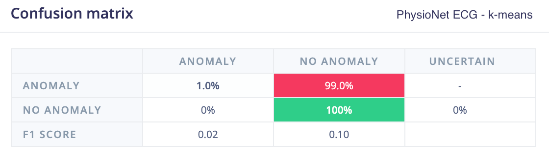
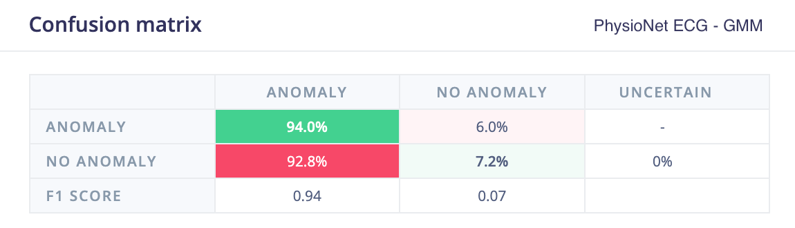
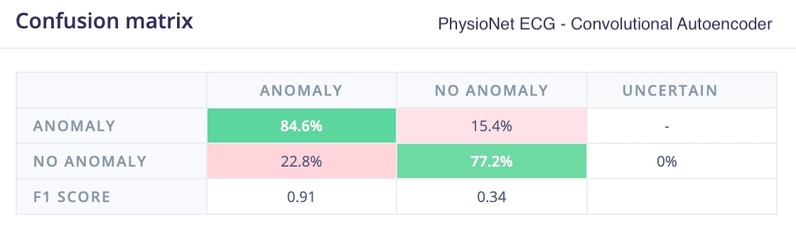
A PhysioNet ECG dataset was used for evaluation, consisting of three classes: NSR (normal sinus rhythm), ARR (arrhythmia), and CFH (congestive heart failure). A single-lead version of the dataset was selected, with NSR samples used for training (reserving a small portion for testing), while ARR and CFH samples were treated as anomalies during testing.
Even with a straightforward initial training run, without extensive hyperparameter tuning, the 1D convolutional autoencoder model achieved strong results and significantly outperformed k-means and GMM models trained on spectral analysis features.
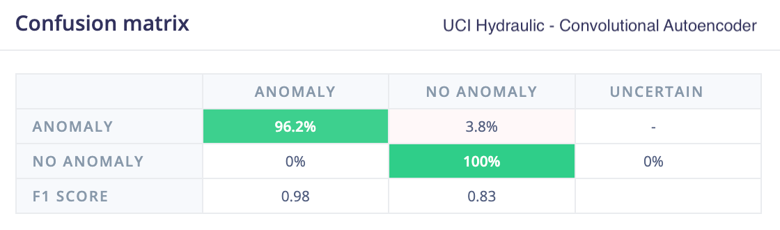
UCI hydraulic press
The UC Irvine condition monitoring of hydraulic systems dataset was used as a the second test dataset. This dataset labels different failure modes, and in this evaluation only the pressure sensor data was used, where subtle variations indicate specific failure conditions.
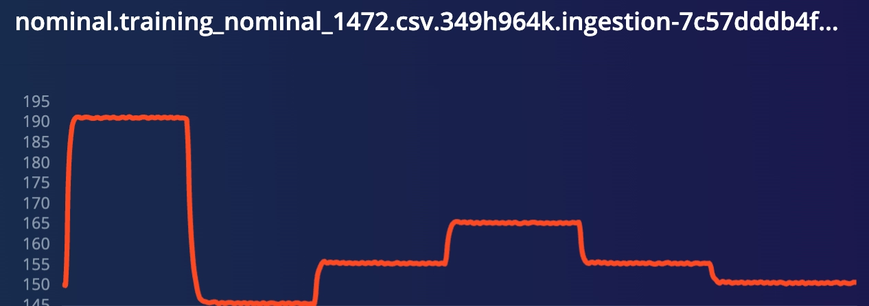
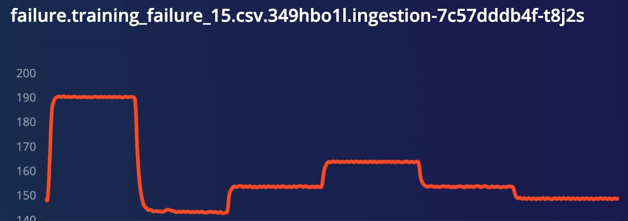
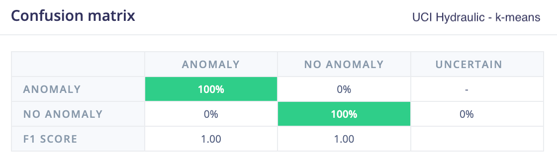
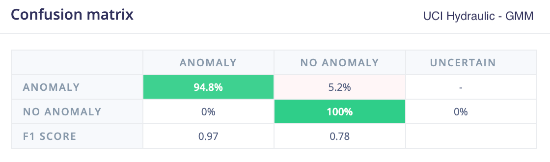
For this dataset, k-means, GMM, and the 1D convolutional autoencoder all performed well at identifying anomalies. This is likely because the spectral analysis features used by k-means and GMM were able to capture the subtle frequency changes that indicated failure.
This also highlights the role of feature quality in clustering-based approaches. Their performance here depends on the spectral features successfully capturing the relevant signal characteristics. In contrast, the convolutional autoencoder achieved comparable results by learning patterns directly from the raw signal, without relying on a separate feature extraction step.
Ultimately, as with most machine learning problems, the right approach depends on your data and constraints. In this case, multiple methods performed well, providing viable options depending on the desired workflow and complexity.
Try it yourself
If you’ve made it this far, the next step is to try it on your own data. If you don’t yet have an Edge Impulse account, you can sign up for free.
Although the convolutional autoencoder was originally developed as a custom learning block, it has since been incorporated directly into the Edge Impulse platform. Based on feedback and usage, we’ve made it available out of the box so anyone can start using it without additional setup.
To get started, create a new project, upload or collect your time-series data, and build your impulse as you normally would. For the learning block, simply select the Anomaly Detection option. After saving your impulse, you’ll find the convolutional autoencoder available on the anomaly detection block configuration page under the neural network architecture section.
You can now experiment with anomaly detection models that go beyond traditional clustering approaches. As additional models are added, you’ll be able to switch between them using the Choose a different model option.
If you’re interested in how the model works under the hood, or want to modify or extend the approach, the full implementation is available in a public GitHub repository. This can serve as a starting point for developing and deploying your own custom anomaly detection blocks. For more details, see:
- Repository: learning-block-autoencoder-ad
- Documentation: Custom learning blocks
This approach is especially useful when working with data where traditional methods don’t fully capture the behavior you’re trying to model.
And if you build something interesting, we’d love to see it. Share your projects, ask questions, or get feedback from the community in our forum and Discord server.